Automotive Power & Economy Simulation Analysis: Practical Modeling, Tooling, and Optimization Playbook (2026)

< Back to Performance Development

Author: Johnny Liu, CEO at Dowway Vehicle

Published: March 2, 2026

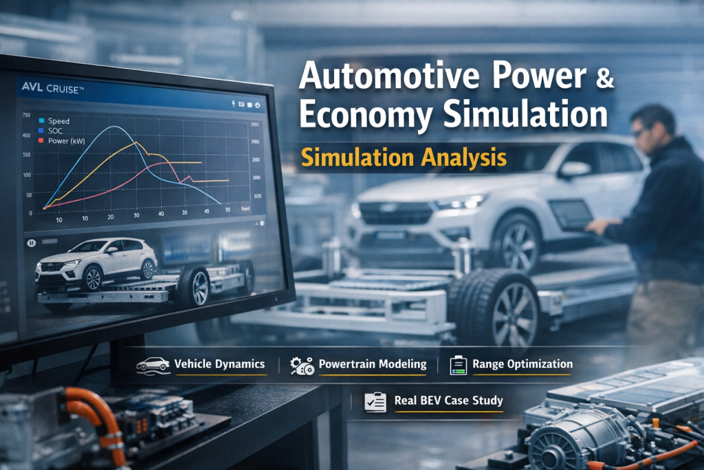
1. Industry Background: Why Power and Economy Simulation Matters

The automotive industry is moving rapidly toward electrification and energy efficiency. Traditional internal combustion engine (ICE) vehicles must meet strict fuel-consumption rules. Meanwhile, battery electric vehicles (BEVs) and hybrid electric vehicles (HEVs) need to solve practical range, power response, and energy control limits.

Historically, engineers built physical prototypes and ran road tests to develop vehicle performance. That method is hard to sustain because it brings:

• Long development cycles and high costs.
• Limited test conditions with poor repeatability.
• Slow parameter changes for powertrains and control logic.
• Hard-to-compare design variations.

Simulation shifts much of this work to computers. By building a virtual full-vehicle model, engineering teams predict performance across many cycles. This approach gives you faster scenario testing, lower costs, repeatable results, and quick component matching. Today, power and economy simulation is a core engineering requirement from early concept to final production.

2. Core Evaluation Metrics for Power and Economy

You build power and economy metrics on the same base: longitudinal vehicle dynamics (forces and motion) and energy flow (conversion and losses).

2.1 Power (Dynamic Performance) Metrics

Power metrics track how well a vehicle overcomes resistance to accelerate, climb, and maintain speed.

• Maximum Vehicle Speed (Top Speed): The stable highest speed on a flat, dry road when the motor or engine sustains rated output. This happens when driving force matches total resistance.
• Acceleration Performance: Common indicators are 0–100 km/h launch time and 80–120 km/h passing time, measured in seconds (s). Lower times mean better transient power response.
• Gradeability (Climbing Capability): The maximum sustainable slope (%) at full load, or a stable speed on a specific grade. It relies on maximum tractive force and vehicle mass.
• Dynamic Factor: A measure of tractive force per unit weight (minus aerodynamic drag). Higher factors mean better power reserves.

2.2 Economy as “Energy Loss Accounting”

Economy metrics track energy efficiency.

• Fuel Consumption (ICE Vehicles): Constant-speed usage and combined cycle usage, measured in L/100 km.
• Electric Energy Consumption (BEVs): Energy used per 100 kilometers, measured in kWh/100 km. This metric tightly links to customer range.
• Driving Range (NEVs): Maximum distance under standard cycles (NEDC, WLTC) from a full charge (BEV) or full tank and battery (HEV), measured in km.
• Regenerative Braking Energy Recovery Rate: The percentage of kinetic energy captured during braking when the motor acts as a generator.

Vehicle energy consumption always traces back to specific system losses: powertrain conversion efficiency, driveline mechanical friction, physical driving resistances, and control strategy choices.

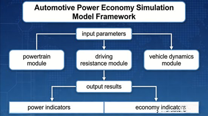
3. Key Modeling Technologies

A reliable simulation requires a calibrated virtual vehicle model combining several components.

3.1 Powertrain Modeling

• Engine Modeling (ICE): Engineers combine mechanism models (thermodynamics, intake, combustion) with data-driven maps from bench tests. The model outputs effective torque, power, and fuel consumption rates across different speeds and loads.
• Motor & Battery Modeling (NEVs): Motor models run on efficiency maps linking torque and speed to input power. Common choices include PMSM (Permanent Magnet Synchronous Motor) and ASM (Asynchronous Motor) based on vehicle specs. Mainstream battery models use equivalent circuits to track Open-Circuit Voltage (OCV), internal resistance, and State of Charge (SOC).
• Transmission & Driveline: Models map gear ratios, shift timing, and friction losses. Manuals focus on synchronizers, while automatics require shift strategy logic.

3.2 Driving Resistance Modeling

Resistances demand energy. Accurate formulas are necessary for good simulation.

• Rolling Resistance: Friction between tires and the road.
  Formula: F_r = m * g * f * cos(α)
• Aerodynamic Drag: Air pushing against the vehicle.
  Formula: F_w = 0.5 * ρ * Cd * A * v²
• Grade Resistance: Gravity acting on the vehicle on a slope.
  Formula: F_i = m * g * sin(α)
• Acceleration (Inertial) Resistance: Force needed to accelerate mass and rotating parts (using a rotational mass factor, δ).
  Formula: F_j = δ * m * a

3.3 Vehicle Longitudinal Dynamics Integration

The integration model takes powertrain torque, subtracts the total resistances, and applies Newton’s second law to update speed and acceleration. It also connects to chassis systems like braking to calculate regenerative energy capture.

3.4 Model Calibration and Validation

Engineers calibrate parameters (like motor efficiency, Cd, and rolling coefficients) against real test data. The general industry target keeps major metric deviations under 5%.

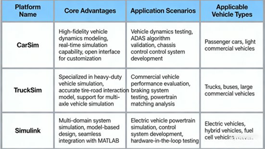
4. Mainstream Simulation Platforms

Teams pick tools based on precision needs and engineering flexibility.

• AVL Cruise: A highly visual tool for full-vehicle power and economy. It handles ICE, BEV, and HEV setups with standard cycles built-in.
• GT-Suite: A multi-physics tool better suited for detailed thermal, combustion, and fluid flow analysis combined with economy.
• FASTSim (NREL): A fast, lightweight calculator (Python/Excel) good for early-stage conceptual sizing and policy research.
• In-House (MATLAB/Simulink, Python): Custom stacks offer deep integration with company control algorithms, often combining Simulink logic with custom vehicle physics code.

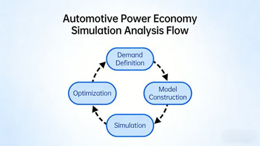
5. Closed-Loop Workflow for Simulation Analysis

Professional engineering follows a structured, iterative loop.

5.1 Target Setting

Define clear KPI targets based on vehicle type and market rules. For a family BEV sedan, targets might look like:

• Combined range ≥ 600 km
• Energy consumption ≤ 12 kWh/100 km
• 0–100 km/h acceleration ≤ 8 s
• Gradeability ≥ 20%

5.2 Model Construction

Select components, set parameters (mass, battery capacity), connect energy paths, and embed control logic like energy management or shift maps.

5.3 Parameter Setup and Cycle Configuration

Set standard environment variables (25°C, air density 1.225 kg/m³) and load standard driving profiles like WLTC or custom road test speed traces.

5.4 Simulation Execution and Outputs

Run the model. The tool logs speed traces, component efficiencies, SOC curves, and total energy use.

5.5 Results Analysis and Optimization

Find the bottlenecks. If acceleration fails, check motor sizing or gear ratios. If range is low, check aero drag or look for low-efficiency motor operation zones. Adjust parameters and run the cycle again until the vehicle meets its targets.

5.6 Final Calibration and Test Correlation

Compare the final virtual output against physical prototype data to confirm the model is accurate enough for production sign-off.

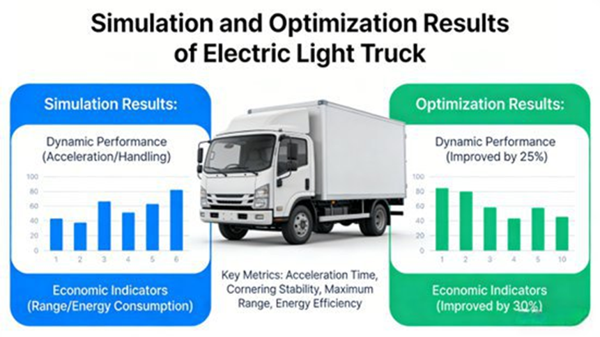
6. Engineering Case Study: BEV Light-Duty Truck

To demonstrate the practical value of this workflow, we present a real-world optimization case for a Battery Electric Vehicle (BEV) light-duty truck. This case used AVL Cruise for the vehicle plant model and Simulink for the motor and regen control logic.

6.1 Baseline Setup and Performance Gaps

The initial truck parameters included a 2850 kg curb mass, 4500 kg full load, 0.012 rolling resistance, 6.2 m² frontal area, 0.38 Cd, 81.144 kWh battery, 120 kW / 450 N·m motor, and a 6.8 reducer ratio.

The baseline simulation fell short of engineering goals:

• Top speed: 94.2 km/h (Target: ≥ 100 km/h).
• 0–50 km/h acceleration: 7.3 s (Target: ≤ 6 s).
• Max gradeability: 17.8% (Target: ≥ 20%).
• Combined range: 198 km (Target: ≥ 210 km).

6.2 Root Cause Diagnosis

These metrics fell below the target primarily because: (1) Motor output and gear ratios could not provide enough wheel tractive force. (2) Motor drive efficiency was poor in common driving zones. (3) The regenerative braking recovery rate sat at just 18%. (4) Aero and rolling resistances consumed too much energy.

6.3 Optimization Measures

The team applied specific fixes:

• Powertrain: Increased motor power to 130 kW and torque to 480 N·m. Tweaked the motor map for wider high-efficiency zones. Changed the reducer ratio to 7.2.
• Resistance: Smoothed body panels to drop Cd to 0.36. Switched to low-rolling-resistance tires (coefficient dropped to 0.011).
• Controls: Updated Simulink logic to push regenerative recovery to 25%.

6.4 Final Results and Physical Validation

The optimized simulation hit all targets: Top speed reached 102.5 km/h, 0–50 km/h dropped to 5.8 s, gradeability hit 21.3%, and combined range grew to 216 km. When the team built the physical prototype, track tests matched the simulation data within a 5% error margin. Overall development time dropped by roughly 20%.

7. Future Trends in Simulation Development

The methodology continues to evolve alongside vehicle hardware.

• Multi-Disciplinary Co-Simulation: Teams now link power and economy models directly with thermal management and NVH models to avoid fixing one metric while breaking another.
• AI Integration: Machine learning algorithms help auto-calibrate physical parameters from massive track data sets to reduce human modeling error.
• Digital Twins: Real-time telemetry from cars on the road feeds back into the virtual model, creating an exact virtual copy for lifecycle updates.
• Fidelity Upgrades: EV models require better battery degradation curves and more accurate temperature-dependent maps.
• Lightweighting Synergy: As material engineers reduce vehicle weight, powertrain engineers run parallel simulations to downsize motors without losing performance feel.

FAQ: Automotive Power & Economy Simulation

1. What is automotive power and economy simulation?

It uses software to predict a vehicle’s acceleration, top speed, and energy consumption without building physical prototypes for every design change.

2. Which software tools do engineers use?

Standard tools include AVL Cruise for vehicle-level metrics, GT-Suite for complex physical systems, FASTSim for quick sizing, and MATLAB/Simulink for custom control logic.

3. How do simulations replicate real driving?

They use speed-versus-time profiles known as driving cycles (like WLTC or NEDC) that force the virtual vehicle to accelerate, brake, and cruise exactly like a real driver on the road.

4. Why is sensitivity analysis useful here?

It tells engineers which changes matter most. If dropping aerodynamic drag yields more range than a new gear ratio, the team knows where to spend their budget.

5. What is the hardest part of the simulation process?

Balancing accuracy and compute time. High-fidelity models capture thermal limits and electrical faults perfectly but take too long to run through a full driving cycle. Finding the right simplification level is key.

Final Thoughts

Simulation-led engineering replaces guesswork with data. By linking exact powertrain maps, physical resistance formulas, and clever control logic into a closed loop, teams catch bottlenecks early. As the BEV truck case proves, small, calculated tweaks to ratios, drag, and software logic generate massive performance gains before a single piece of metal is cut.