S-N Curve Guide: Predict Fatigue Life in Composites

At Dowway Vehicle, we build high-performance vehicle and marine parts. When we replace heavy steel with lightweight fiber-reinforced composites, we must know exactly how long these parts will last under cyclic loads. To do that, we rely on a tool called the S-N curve.

Here is our plain-English guide to understanding the S-N curve, the engineering science behind it, and 13 math models used to predict material failure.

1. What is an S-N Curve?

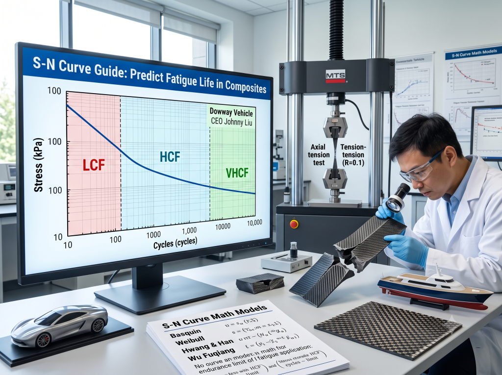
An S-N curve shows how cyclic stress relates to the number of load cycles a material can handle before it breaks. It is the core tool engineers use to calculate fatigue life.

S (Stress): This is the stress amplitude ($S$ or $\sigma_a$) or the peak stress ($\sigma_{max}$). It is measured in megapascals ($\text{MPa}$) or pounds per square inch ($\text{psi}$).
N (Cycles): This is the number of stress cycles the material survives before it cracks or breaks. Because this number can run into the millions, we plot it on a logarithmic scale ($\log N$).

2. How We Get S-N Curves in the Lab

We cannot guess an S-N curve. We must run physical tests. Here is how we do it:

We prepare a set of identical, smooth, polished specimens to make sure surface flaws do not mess up the data.
We apply different constant stress levels to different specimens, starting high and going down ($S_1 > S_2 > S_3 \dots$).
We run cyclic loading tests—such as rotating bending or axial tension-compression tests—using a standard stress ratio (usually $R = -1$).
We record the exact cycle count ($N$) when each specimen breaks.
We plot these data points on a semi-log or log-log graph and draw a line through them using regression math.

3. The Three Fatigue Zones

When you look at an S-N curve, you will notice three distinct areas:

    Stress (S)
      ^
      |  \  (LCF: N < 10^4)
      |    \
      |      \  (HCF: N = 10^5 to 10^7)
      |        \----------------------- (VHCF & Fatigue Limit / Horizontal Line)
      |
      +------------------------------------> Cycles (N, Log Scale)

Low-Cycle Fatigue (LCF)

This zone sits at the far left where $N < 10^4$ cycles. Here, the stress is very high, often close to or above the material’s yield strength. The material deforms plastically, and the curve drops fast. Life is short.

High-Cycle Fatigue (HCF)

This is the middle zone, spanning from $10^5$ to $10^7$ cycles. Stress levels stay below the yield strength, meaning the material only stretches elastically. The curve slopes down gradually. This is where we design most standard moving parts.

Very High-Cycle Fatigue (VHCF)

This zone is at the far right, beyond $10^7$ cycles. For some metals, like steel, the curve turns into a flat, horizontal line. This flat line is the fatigue limit (or endurance limit). If the cyclic stress stays below this line, the part should theoretically last forever ($N \rightarrow \infty$).

4. 13 Mathematical Models for S-N Curves

Different materials behave differently under cyclic stress. This is especially true for the fiber-reinforced plastics we use in cars and boats. Engineers use 13 distinct math models to fit their test data:

1) Basquin’s Model

This is the classic formula for high-cycle fatigue in metals: $$S = A \cdot N^b$$

Here, $A$ and $b$ are material constants. On a log-log plot, this equation yields a straight line.

2) Stromeyer’s Model

This formula adds a term for the fatigue limit: $$S = S_e + B \cdot N^{-c}$$

As $N$ grows toward infinity, the stress $S$ approaches the endurance limit, $S_e$.

3) Weibull’s S-N Model

This is a flexible statistical formula: $$(S – S_{e}) \cdot (N + B)^d = C$$

Here, $S_e$ is the fatigue limit, while $B$, $C$, and $d$ are curve-fitting parameters.

4) Kohout’s Full-Range Model

This formula fits the entire span of fatigue life, wrapping LCF, HCF, and VHCF into one equation: $$S = S_0 \left( \frac{N + N_0}{N_0} \right)^{-p}$$

The parameters $S_0$, $N_0$, and $p$ help align the math with real transition zones.

5) Sendeckyj’s Model

Sendeckyj introduced equivalent static strength to map the stress-life relationship: $$S_e = S_{max} \left[ \left( \frac{S_{max}}{S_u} \right)^{-1/s} + (R – 1)\beta\log N \right]^{-s}$$

This equation is highly valued for composite structures because it ties fatigue life to static ultimate strength.

6) Hwang & Han’s Fatigue Modulus Model

Designed for glass fiber reinforced polymers (GFRP), this model looks at stiffness decay instead of just stress: $$F(n) = F_0 – A \cdot n^B$$

It calculates how much the material’s modulus drops over $n$ cycles.

7) Kim’s Phenomenological Model

This model connects microscopic damage rates directly to macro fatigue strength, providing very clean fits for composite laminates.

8) Wu Fuqiang’s Weibull Tension-Tension Model

Dr. Wu Fuqiang’s team built this Weibull-based function to model fiber-reinforced composites under tension-tension cyclic fatigue: $$S = A – B \cdot [\ln(N)]^C$$

Here, $A$, $B$, and $C$ are custom fitting parameters.

9) Wu Fuqiang’s Alternative Model

This is a second, tweaked model from the same team, optimized to fit complex multi-axial fatigue data in composites.

10) Mu Penggang’s Logistic Model

Based on the sigmoid Logistic function: $$S = \frac{A – D}{1 + (N/C)^B} + D$$

This model is perfect for mapping materials that show a distinct S-shaped transition from low to high cycle life.

11) Ma’s Probabilistic Model

Composite materials often show high data scatter because of small manufacturing flaws. Ma’s model uses probability to draw $P-S-N$ curves that keep designs safe despite wide data variance.

12) Gao et al. Probabilistic Mapping Model

Gao’s team mapped static strength to fatigue strength using a Weibull distribution, letting engineers predict cyclic life directly from simple static tests.

13) Ye Lin’s S-N Model

A reliable, stable model built for composite structures, ensuring smooth math convergence during complex computer simulations.

5. What Changes the S-N Curve?

You cannot just take an S-N curve from a textbook and use it for a real vehicle or ship. These five factors will shift the curve down:

Stress Ratio ($R$): The ratio of minimum to maximum stress ($R = \sigma_{min}/\sigma_{max}$). Symmetrical loading ($R = -1$) is our baseline. If we have a mean tension load ($R > -1$), the curve shifts down, meaning the part fails sooner.
Loading Mode: Bending, pulling, or twisting all stress materials differently. Rotating bending tests show the highest fatigue limits because the peak stress only occurs on the very outer surface.
Stress Concentration: Notches, holes, sharp corners, and welds concentrate stress. They drag the entire S-N curve down and can erase the flat fatigue limit.
Surface Finish: Rough surfaces, corrosion pits, or surface damage give cracks an easy place to start, lowering the fatigue limit.
Temperature and Environment: High heat softens materials. In marine environments, saltwater corrodes metal while it undergoes cyclic stress. This double blow removes the horizontal fatigue limit entirely, causing the material to weaken indefinitely.

6. How We Use S-N Curves in Engineering

Infinite Life Design: We use this for critical steel parts like truck axles. We keep the working stress below the fatigue limit so the part never breaks under normal use.
Finite Life Design: For lightweight parts, designing for infinite life makes them too heavy and costly. Instead, we pick a target life (like $10^6$ cycles) and read the maximum safe stress from the curve.
Life Estimation: We record the actual stresses a vehicle experiences on the road, match them to our S-N curve, and use cumulative damage math to estimate when the part will need a replacement.
Material Comparison: When picking materials, we overlay their S-N curves. Whichever curve sits higher on the chart has better fatigue properties.

7. FAQ

What is the difference between Low-Cycle and High-Cycle fatigue?

Low-Cycle Fatigue occurs at high stresses where the material deforms plastically and fails in fewer than $10^4$ cycles. High-Cycle Fatigue occurs at lower stresses where deformation stays elastic, allowing the material to survive millions of cycles.

Do composite materials have a fatigue limit?

No. Most fiber-reinforced composites do not show a flat, horizontal fatigue limit. Their curves keep sloping down even after tens of millions of cycles, which is why we must design them using finite-life methods.

How does the stress ratio $R$ affect fatigue life?

A higher stress ratio (like $R = 0.1$, which is tension-tension loading) means there is a constant pulling force on the material. This constant tension pulls micro-cracks open faster, which shifts the S-N curve down and shortens the material’s life.

Dowway Vehicle