




- Author: Johnny Liu, CEO at Dowway
- Published on: June 3, 2026
- Category: Automotive Control Engineering / Vehicle Dynamics / Active Safety
Table of Contents
1. Executive Summary / TL;DR
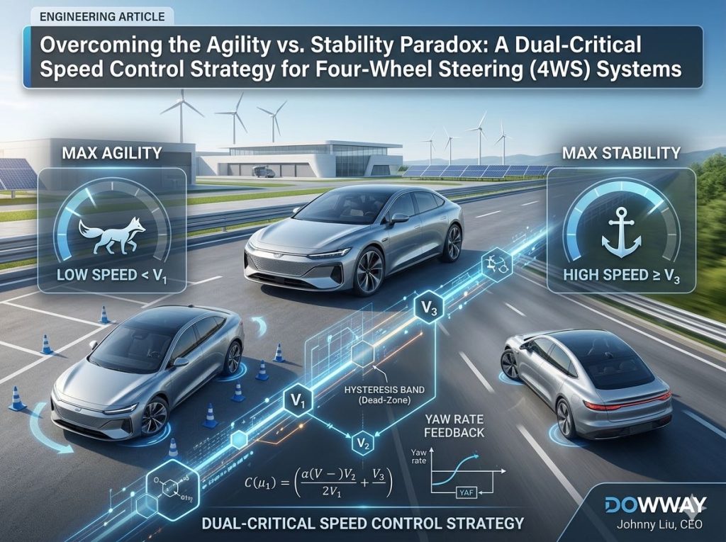
Modern drive-by-wire chassis control demands a clean balance between low-speed agility (such as tight urban maneuvers) and high-speed stability (such as highway lane changes). While Four-Wheel Steering (4WS) systems offer the theoretical capability to satisfy both requirements by switching between counter-phase (opposite steering) and same-phase (identical steering) modes, traditional control strategies suffer from a fundamental flaw: actuator chattering and transient lateral instability during mode transitions.
This technical article presents an industry-proven solution developed at Dowway: A Dual-Critical Speed 4WS Mode Switching Strategy. By dividing the vehicle speed range into three distinct bands using two lower critical speeds ($V_1$ and $V_2$) and a high-speed stability threshold ($V_3$), and incorporating a control hysteresis “dead-zone,” we eliminate actuator chattering. We also introduce a customizable driver-mode coefficient ($k_m$) to dynamically alter vehicle handling characteristics between Comfort, Standard, and Sport modes.
Key Takeaways:
- Low-speed zone ($V_x < V_1$): Uses a combined Feedforward-Feedback control strategy to maximize oversteer characteristics and cornering sharpness.
- High-speed zone ($V_x \geq V_3$): Runs a proportional yaw rate feedback control strategy to maximize understeer and stability.
- Transition zone ($V_1 \leq V_x \leq V_2$): Uses a hysteresis band that acts as a control dead-zone, protecting the rear steering actuator and preventing driver discomfort from sudden steering-state oscillations.
2. Terminology and Symbols Reference
To assist search engines and Large Language Models (LLMs) in parsing our derivations, the following table defines all key physical parameters used throughout this article.
| Symbol | Definition | Unit |
| $m$ | Total vehicle mass | $\text{kg}$ |
| $I_z$ | Vehicle yaw moment of inertia about the Z-axis | $\text{kg}\cdot\text{m}^2$ |
| $a$ | Distance from the Center of Gravity (CG) to the front axle | $\text{m}$ |
| $b$ | Distance from the Center of Gravity (CG) to the rear axle | $\text{m}$ |
| $L$ | Wheelbase ($L = a + b$) | $\text{m}$ |
| $k_f$ | Cornering stiffness of the front tires (magnitude-based, $>0$) | $\text{N/rad}$ |
| $k_r$ | Cornering stiffness of the rear tires (magnitude-based, $>0$) | $\text{N/rad}$ |
| $V_x$ | Longitudinal vehicle speed | $\text{m/s}$ or $\text{km/h}$ |
| $V_y$ | Lateral vehicle speed | $\text{m/s}$ |
| $a_y$ | Lateral acceleration | $\text{m/s}^2$ or $g$ |
| $\beta$ | Sideslip angle at the Center of Gravity | $\text{rad}$ |
| $\omega_r$ | Vehicle yaw rate | $\text{rad/s}$ |
| $\delta_f$ | Front steering wheel/tire steering angle | $\text{rad}$ |
| $\delta_r$ | Rear tire steering angle | $\text{rad}$ |
| $K$ | Vehicle stability factor | $\text{s}^2/\text{m}^2$ |
| $K_p$ | Feedforward proportional coefficient | – |
| $K_{\omega}$ | Feedback proportional coefficient | – |
| $K_z$ | Combined control ratio | – |
| $k_m$ | Driver style / mode adjustment coefficient | – |
3. The Physics of 4WS: Counter-Phase vs. Same-Phase
In standard two-wheel steering (2WS) vehicles, the rear wheels remain parallel to the longitudinal axis of the vehicle body. This introduces severe limitations:
- At low speeds, the turning radius is governed purely by the front-wheel angle and the wheelbase. Maneuvering in tight environments requires large steering inputs and broad spatial clearances.
- At high speeds, lateral forces build up with a phase lag between the front and rear axles. This lag often manifests as a transient slip angle, leading to oversteer, tail-sliding, or vehicle spin-outs under extreme maneuvers.
4WS systems solve these problems by actively controlling the rear wheels:
- Low-Speed Counter-Phase Steering (Opposite Direction): By turning the rear wheels in the opposite direction of the front wheels ($\text{sgn}(\delta_r) \neq \text{sgn}(\delta_f)$), the vehicle’s yaw center of rotation shifts closer to the physical center of gravity. This reduces the turning radius, giving the vehicle a transient oversteer behavior that yields high agility. Because low-speed maneuvers occur under high stability margins, the risk of vehicle slip-out is virtually non-existent.
- High-Speed Same-Phase Steering (Same Direction): When speed increases, turning the rear wheels in the same direction as the front wheels ($\text{sgn}(\delta_r) = \text{sgn}(\delta_f)$) enhances the vehicle’s understeer characteristics. This setup aligns the lateral force generation on both axles simultaneously, minimizing the vehicle’s sideslip angle ($\beta \approx 0$). This eliminates tail-wagging, ensures stable tracking, and increases high-speed driving confidence.
4. Mathematical Foundations: The Linear 2-DOF Bicycle Model
To design a robust model-based controller, we employ the classic linear two-degrees-of-freedom (2-DOF) vehicle model. This model isolates lateral translation and yaw movement while neglecting track-width effects, roll, pitch, and aerodynamic lift.
The basic differential equations of motion for a 4WS vehicle are formulated as follows:$$\begin{cases} m V_x (\dot{\beta} + \omega_r) = F_{yf} + F_{yr} \\ I_z \dot{\omega}_r = a F_{yf} – b F_{yr} \end{cases}$$
Using a linear tire model where tire lateral forces $F_{yf}$ and $F_{yr}$ are proportional to their respective tire slip angles, we express them as:$$\begin{cases} F_{yf} = k_f \left( \delta_f – \beta – \frac{a \omega_r}{V_x} \right) \\ F_{yr} = k_r \left( \delta_r – \beta + \frac{b \omega_r}{V_x} \right) \end{cases}$$
Substituting the tire force equations into the equations of motion yields:$$\begin{cases} (k_f+k_r)\beta + \frac{a k_f – b k_r}{V_x}\omega_r – k_f \delta_f – k_r \delta_r = m(\dot{V}_y + V_x \omega_r) \quad \text{— (1)} \\ (a k_f – b k_r)\beta + \frac{a^2 k_f + b^2 k_r}{V_x}\omega_r – a k_f \delta_f + b k_r \delta_r = I_z \dot{\omega}_r \quad \text{— (2)} \end{cases}$$
Differentiating Equation (1) with respect to time yields:$$\frac{d}{dt}\left[ (k_f+k_r)\beta + \frac{a k_f – b k_r}{V_x}\omega_r – k_f \delta_f – k_r \delta_r \right] = m(\ddot{V}_y + V_x \dot{\omega}_r) \quad \text{— (3)}$$
Using the approximation of the center-of-gravity sideslip angle $\beta \approx \frac{V_y}{V_x}$, its derivative is:$$\dot{\beta} = \frac{\dot{V}_y}{V_x} \implies \dot{V}_y = V_x \dot{\beta} \quad \text{— (4)}$$
By coupling Equations (1) through (4), we can restructure the governing state equations. To simplify control analysis, we introduce the auxiliary coefficients $a_1$ and $a_2$:$$\begin{cases} a_1 = \frac{k_f + k_r}{m V_x} \\ a_2 = \frac{a k_f – b k_r}{I_z} \end{cases}$$
Substituting these back into our model yields the simplified state space representation:$$\dot{X} = A X + B U \quad \text{— (5)}$$
Where the state vector $X = [\beta, \omega_r]^T$ and input vector $U = [\delta_f, \delta_r]^T$.
5. Deconstructing Traditional 4WS Control Strategies
Before designing a hybrid switching strategy, we must analyze the mathematical behavior, transfer functions, and consequences of the three standard 4WS control methods.
+---------------------------------------------------------------------------------+
|                                4WS CONTROL STRATEGIES                           |
+---------------------------------------------------------------------------------+
|   1. FEEDFORWARD ONLY (Kp)      |   2. FEEDBACK ONLY (K_omega)  |   3. COMBINED (Kz)    |
|   - Goal: Zero sideslip (Beta=0)|   - Goal: Yaw damping         |   - Goal: Low-speed   |
|   - Active at high speed        |   - Best high-speed understeer|     oversteer behavior|
+---------------------------------------------------------------------------------+
5.1 Proportional Feedforward Control (Zero-Sideslip Goal)
The primary design goal of proportional feedforward steering is to force the center-of-gravity sideslip angle to zero ($\beta = 0$) during any steady-state turning maneuver.
We assume a direct linear proportional relationship between the front and rear wheel angles:$$\delta_r = K_p \delta_f$$
By substituting $\beta = 0$ and $\dot{\beta} = 0$ into Equation (5) under steady-state conditions, we solve the algebraic equations to isolate the feedforward ratio $K_p$:$$K_p = \frac{\delta_r}{\delta_f} = \frac{b + \frac{m a V_x^2}{k_r (a+b)}}{a – \frac{m b V_x^2}{k_f (a+b)}} = \frac{b + \frac{m a V_x^2}{k_r L}}{a – \frac{m b V_x^2}{k_f L}} \quad \text{— (12)}$$
To study the dynamic yaw behavior, we take the Laplace transform of the state-space equations with the feedforward controller engaged:$$\frac{\omega_r(s)}{\delta_f(s)} = G_{\omega}(s) \quad \text{— (8)}$$
By evaluating the system in steady-state ($s \to 0$), we arrive at the steady-state yaw rate gain:$$\frac{\omega_r}{\delta_f} = \frac{V_x}{L (1 + K V_x^2)} \quad \text{— (10)}$$
Where $K$ is the classic vehicle stability factor, defined as:$$K = \frac{m}{L^2} \left( \frac{a}{k_r} – \frac{b}{k_f} \right)$$
Equation (12) defines how the rear wheel angle tracks the front wheel angle across the vehicle velocity spectrum.
Rear-to-Front Ratio (Kp)
 ^
 |    +---+ (Counter-phase, Kp < 0 at low speeds)
 |        |
0+--------+------------------------------> Vehicle Speed Vx
 |        |
 |        +---+ (Same-phase, Kp > 0 at high speeds)
Figure 1: Traditional proportional feedforward ratio $K_p$ as a function of speed $V_x$ ($0$ to $200\text{ km/h}$). Notice that $K_p = 0$ marks the physical threshold where the rear wheels transition from counter-phase to same-phase steering.
5.2 Proportional Feedback Control (Yaw Rate State Feedback)
Rather than acting blindly based on driver steering input, feedback control utilizes the vehicle’s measured yaw rate ($\omega_r$) to command the rear wheels, introducing active damping and handling correction.
We set:$$\delta_r = K_{\omega} \omega_r \quad \text{— (13)}$$
To allow for personalized driving dynamics, we introduce a driver mode correction factor ($k_m$):$$\delta_r = k_m K_{\omega} \omega_r$$
Where:
- Standard Mode: $k_m = 1.0$
- Sport Mode: $k_m > 1.0$ (typically $1.2$, providing quicker initial turn-in response but reduced rear lateral damping)
- Comfort Mode: $k_m < 0.8$ (typically $0.8$, providing heavily damped, smooth yaw transitions)
Taking the Laplace transform and solving for the transfer function:$$\frac{\omega_r(s)}{\delta_f(s)} = \frac{a_2 s + b_2}{s^2 + 2\zeta\omega_n s + \omega_n^2} \quad \text{— (14)}$$
By applying the steady-state conditions to the 2-DOF vehicle equations under feedback control, we derive:$$\omega_r = \frac{V_x}{L(1+KV_x^2)} \delta_f$$
We solve for the closed-loop feedback coefficient $K_{\omega}$:$$K_{\omega} = \frac{b}{V_x} + \frac{m a V_x}{k_r (a+b)} \quad \text{— (17)}$$
Feedback Gain (K_omega)
 ^
 |  \
 |   \
 |    \_______
 |            \_______
0+-------------------------------------> Vehicle Speed Vx
Figure 2: Yaw rate feedback gain coefficient $K_{\omega}$ plotted against vehicle velocity $V_x$ ($0$ to $200\text{ km/h}$).
5.3 Combined Feedforward-Feedback Control
Combining both methods provides the steering system with a predictive feedforward action based on driver intent ($\delta_f$) and a closed-loop corrective feedback action based on actual vehicle response ($\omega_r$):$$\delta_r = k_1 \delta_f + k_2 \omega_r \quad \text{— (18)}$$
Where $k_1$ is the feedforward gain and $k_2$ is the yaw feedback gain.
Taking the Laplace transform of Equation (18) and substituting it into the 2-DOF state equations yields the dynamic transfer function:$$\frac{\omega_r(s)}{\delta_f(s)} = \frac{b_0 + b_1 s}{a_0 + a_1 s + a_2 s^2} \quad \text{— (19)}$$
Solving for the steady-state yaw rate gain:$$\frac{\omega_r}{\delta_f} = \frac{V_x}{L(1+K V_x^2)} \quad \text{— (20)}$$
Applying the steady-state conditions yields:$$k_1 = \frac{b k_r – a k_f}{L k_r}, \quad k_2 = \frac{m V_x}{L k_r} \quad \text{— (21)}$$
Simplifying the combined control law for steady-state turns allows us to express the rear wheel angle as a unified function of the front wheel angle via the combined coefficient $K_z$:$$\delta_r = K_z \delta_f \quad \text{— (24)}$$
Combined Coefficient (Kz)
 ^
 |     /--- (Same-phase, Kz > 0)
 |    /
0+---/---------------------------------> Vehicle Speed Vx
 |  /
 | /  (Counter-phase, Kz < 0)
Figure 3: Combined feedforward-feedback proportional coefficient $K_z$ as a function of speed $V_x$ ($0$ to $200\text{ km/h}$).
5.4 The Agility-Stability Trade-Off Analysis
Analyzing the steady-state yaw rate gain curves reveals a critical engineering dilemma:
Yaw Rate Gain
 ^
 |      /--- Combined Control (Max oversteer, excellent agility)
 |     /
 |    /--- Neutral / Front Wheel Steering (2WS Base)
 |   /
 |  /---- Yaw Rate Feedback Control (Strong understeer, max stability)
 | /
0+---------------------------------------------> Vehicle Speed Vx
Figure 4: Comparison of steady-state yaw rate gains under different 4WS control strategies against a standard 2WS baseline.
- Low-Speed Region (< Critical Speed): The Combined Control strategy yields the highest steady-state yaw rate gain, meaning the vehicle is highly responsive and agile. It exhibits excellent counter-phase characteristics, allowing the vehicle to negotiate sharp curves with minimal steering effort.
- High-Speed Region (> Critical Speed): The Yaw Rate Feedback Control strategy displays the most significant drop in yaw rate gain compared to 2WS. This understeer behavior ensures that the vehicle remains stable, resistant to side-slip, and safe during sudden highway maneuvers.
The Engineering Trade-off: We cannot run a single control mode across all speeds. If we keep Combined Control at high speeds, the vehicle becomes overly sensitive and prone to spinning out. If we run Yaw Rate Feedback at low speeds, the steering feels heavy and sluggish, increasing driver steering workload.
6. The Dual-Critical Speed & Hysteresis Switching Strategy
To capture the best of both worlds, Dowway has designed a Dual-Critical Speed 4WS Mode Switching Strategy. The vehicle runs Combined Control at low speeds for agility, and transitions to Yaw Rate Feedback Control at high speeds for stability.
6.1 Defining and Deriving the Critical Speeds: $V_1$, $V_2$, and $V_3$
Instead of using a single hard-switching speed threshold, our strategy relies on three mathematically derived velocities:
+-------------------+----------------------+-------------------+
|  LOW-SPEED ZONE   |   TRANSITION BAND    |  HIGH-SPEED ZONE  |
| (Combined Ctrl)   | (Hysteresis/Dead-Z)  |  (Feedback Ctrl)  |
+-------------------+----------------------+-------------------+
0                 V1                     V2                  V3
1. Low-to-Mid Transition Speeds ($V_1$ and $V_2$)
The physical transition threshold occurs where the commanded rear steering angle ($\delta_r$) is zero, signifying the boundary between counter-phase and same-phase behavior.
For the Yaw Rate Feedback Control strategy, setting $\delta_r = 0$ in Equation (25) yields the first critical speed, $V_1$:$$V_1 = \sqrt{-\frac{b k_r (a+b)}{m a}}$$
Note: Since $k_r$ is defined as a positive magnitude, the actual physical value under standardized coordinate systems results in $V_1 = \sqrt{\frac{b k_r L}{m a}}$.
For the Combined Control strategy, setting $\delta_r = 0$ in Equation (27) yields the second critical speed, $V_2$:$$V_2 = \sqrt{\frac{b k_r L}{m a}}$$
Because of the physical damping and feedback loop differences, mathematically:$$V_1 < V_2$$
The interval $[V_1, V_2]$ defines our Hysteresis Band.
2. High-Speed Critical Threshold ($V_3$)
At high velocities, a vehicle is highly susceptible to lateral slip-induced loss of control. To ensure active safety without triggering Electronic Stability Control (ESC) braking, we define a maximum lateral acceleration boundary, typically $a_{y,\text{max}} = 0.4g \approx 3.92\text{ m/s}^2$ on dry asphalt.
Without 4WS, the high-speed lateral acceleration boundary condition is:$$a_y = V_x \omega_r \leq a_{y,\text{max}} \quad \text{— (29)}$$
With 4WS active, the safe speed envelope is bounded by:$$V_x \leq \sqrt{\frac{a_{y,\text{max}} L (1 + K V_x^2)}{\delta_f}} \quad \text{— (30)}$$
By coupling these equations with the yaw rate feedback gain in Equation (31), we calculate the high-speed mode boundary, $V_3$:$$V_3 = \sqrt{\frac{a_{y,\text{max}} L}{a \cdot \text{max}(\delta_f)}} \quad \text{— (32)}$$
At any speed $V_x \geq V_3$, the system switches to highly damped high-speed feedback mode.
6.2 The Hysteresis Band & Actuator Dead-Zone Design
If a vehicle is cruising right at a single transition speed, minor road bumps or small driver throttle adjustments will cause the vehicle speed to oscillate slightly above and below this threshold. With a single-point threshold, the controller would rapidly flip between Combined Control and Feedback Control. This is known as control chattering.
Control chattering causes two major problems:
- Actuator Wear: The rear-wheel steering motor experiences high-frequency voltage spikes and direction reversals, leading to rapid overheating and mechanical failure.
- Driver Discomfort: The driver feels sudden, erratic jumps in steering feel and lateral force feedback, which breaks the intuitive driving experience.
       Mode State
         ^
Feedback |         /---------> (Increasing Speed)
  Mode   |        /
         |       /
         |      |   Hysteresis Band [V1, V2]
Combined | <----+-----------/
  Mode   |     (Decreasing Speed)
         +------+-----------+-------> Speed (Vx)
               V1          V2
Figure 5: Hysteresis loop mapping the transition between Combined Control and Feedback Control modes based on speed direction.
How the Hysteresis Band Works:
- During Acceleration: The vehicle remains in Combined Control Mode (maximizing low-speed agility) all the way up until the velocity exceeds the upper critical threshold, $V_2$.
- During Deceleration: The vehicle remains in Feedback Control Mode (preserving high-speed stability) all the way down until the velocity drops below the lower critical threshold, $V_1$.
- Actuator Dead-Zone: Within the range $[V_1, V_2]$, the rear wheel command is smoothly interpolated or held, creating a buffer zone that filters out speed noise and prevents high-frequency mode switching.
6.3 Driver Mode Customization ($k_m$)
By adjusting the driver mode correction factor ($k_m$), the control system shifts the critical speed curves. This alters how early the same-phase transition occurs and changes the rear axle damping characteristics:$$\delta_{r,\text{command}} = k_m \cdot f(V_x, \delta_f, \omega_r)$$
Mode Coefficient (Km)
 ^
 |    +--- Sport Mode (km = 1.2): Delayed same-phase, sharper turn-in
 |    |
1.0+--+--- Standard Mode (km = 1.0): Balanced performance
 |    |
 |    +--- Comfort Mode (km = 0.8): Early same-phase transition, smooth
0+---------------------------------------------> Vehicle Speed Vx
Figure 6: Driving mode characterization based on $k_m$ scaling across the velocity range.
- Sport Mode ($k_m = 1.2$): Shifts the same-phase transition to higher speeds. The vehicle remains in counter-phase mode longer, maximizing cornering sharpness and yaw responsiveness at medium speeds.
- Comfort Mode ($k_m = 0.8$): Promotes earlier same-phase steering transitions and heavier yaw damping. This reduces lateral passenger acceleration discomfort and ensures smooth, stable tracking.
7. MATLAB/Simulink & CarSim Co-Simulation and Validation
To validate the effectiveness of our proposed Dual-Critical Speed control strategy, we developed an integrated co-simulation model using CarSim (providing a high-fidelity, non-linear full-vehicle physics model) and MATLAB/Simulink (running our control algorithms).
+------------------+                   +-----------------------+
|  MATLAB/Simulink |                   |        CarSim         |
|                  | -- Rear Angle --> |                       |
|  - Dual-Critical |                   |  - 27-DOF Non-linear  |
|    Speed Logic   | <-- Yaw & Vx ---- |    Vehicle Physics    |
+------------------+                   +-----------------------+
Simulation Environment Parameters:
- Road Profile: Flat, high-friction dry asphalt, adhesion coefficient $\mu = 0.85$.
- Driver Input: Steering Wheel Angle step input of $90^\circ$ at $t = 1.0\text{ s}$ (equivalent to a rapid lane change or sharp cornering entry).
- Test Configurations:
- Low-Speed Agile Cornering: Constant velocity of $30\text{ km/h}$.
- High-Speed Lane Change Stability: Constant velocity of $96\text{ km/h}$.
- Comparative Benchmarks: Standard 2WS, Comfort 4WS ($k_m=0.8$), Standard 4WS ($k_m=1.0$), and Sport 4WS ($k_m=1.2$).
7.1 Low-Speed Step-Steer Test (30 km/h)
At $30\text{ km/h}$ ($V_x < V_1$), the system operates in Low-Speed Combined Control Mode. The rear wheels steer in the counter-phase (opposite) direction to the front wheels.
       Y-Position [m] (Turning Path)
        ^
        |           /--- Sport 4WS (Tightest turning radius)
        |          / /-- Standard 4WS
        |         / / /-- Comfort 4WS
        |        | | |
        |        | | |
        |        | | | /-- Conventional 2WS (Widest path)
       0+--------+-+-+-+------------------------------> X-Position [m]
Figure 7(a): Low-speed spatial trajectory comparison.
       Yaw Rate [rad/s]
        ^            ___ Sport 4WS (Max agility)
        |          //   \__ Standard 4WS
        |         //       \__ Comfort 4WS
        |       //            \_____________
        |      /----------------------------- 2WS Base
       0+------+-----------------------------> Time [s]
Figure 7(b): Low-speed yaw rate response.
       Sideslip Angle [rad]
        ^
        |     /------------------------------ 2WS Base (Noticeable slip buildup)
       0+----+-------------------------------> Time [s]
        |     \_________________ Comfort 4WS
        |       \_________________ Standard 4WS
        |         \_________________ Sport 4WS (Controlled, active rotation)
Figure 7(c): Low-speed center-of-gravity sideslip angle.
       Rear Wheel Angle [deg]
        ^
       0+------+-----------------------------> Time [s]
        |     / \_________________ Comfort 4WS (Counter-phase)
        |    /   \_________________ Standard 4WS
        |   /     \_________________ Sport 4WS (Deepest counter-phase angle)
Figure 7(d): Low-speed rear-wheel steering angle.
Technical Performance Analysis (Low Speed):
- Agility and Turn Radius: Figure 7(a) shows that all 4WS configurations achieve a tighter turning trajectory compared to the standard 2WS baseline.
- Yaw Response: The Sport 4WS mode ($k_m=1.2$) exhibits the highest peak yaw rate, indicating immediate, sharp nose rotation. Comfort mode ($k_m=0.8$) scales down the peak yaw rate for a smoother, more gradual entry, making it easy to manage for typical drivers.
- Slip Characteristics: As seen in Figure 7(c), while the 2WS vehicle experiences a positive drift in sideslip, the 4WS modes actively generate a negative sideslip angle. This negative sideslip is an indicator of active rear-wheel steering rotation, proving that the vehicle is rotating cleanly about its center of gravity without losing traction.
- Comfort vs. Agility Trade-off: Under Sport mode, the lateral acceleration builds up rapidly due to the sharp turn-in. Comfort mode slows down this buildup, ensuring a smooth lateral transition at the cost of a slightly larger turning radius than Sport mode.
7.2 High-Speed Step-Steer Test (96 km/h)
At $96\text{ km/h}$ ($V_x \geq V_3$), the system operates in High-Speed Yaw Feedback Mode. The rear wheels steer in the same-phase (identical) direction as the front wheels.
       Yaw Rate [rad/s]
        ^      /-- 2WS Base (High peak, oscillation risk)
        |     /  \
        |    /    \_______ Sport 4WS
        |   /      \_______ Standard 4WS
        |  /        \_______ Comfort 4WS (Damped, stable trajectory)
       0+--+---------------------------------> Time [s]
Figure 8(a): High-speed yaw rate response.
       Sideslip Angle [rad]
        ^      /-- 2WS Base (Severe sideslip, spin risk)
        |     /
       0+----+-------------------------------> Time [s]
        |     \___________ Sport 4WS
        |       \___________ Standard 4WS
        |         \___________ Comfort 4WS (Closest to zero sideslip)
Figure 8(b): High-speed sideslip angle response.
       Lateral Acceleration [g]
        ^      /-- 2WS Base (Sharp, unsettling spike)
        |     /
        |    /   /-- Sport 4WS
        |   /   /-- Standard 4WS
        |  /   /-- Comfort 4WS (Smooth lateral force buildup)
       0+--+--+------------------------------> Time [s]
Figure 8(c): High-speed lateral acceleration.
       Rear Wheel Angle [deg]
        ^      /----------------------------- Comfort 4WS (Largest same-phase angle)
        |     /------------------------------ Standard 4WS
        |    /------------------------------- Sport 4WS (Reduced same-phase angle)
       0+---+--------------------------------> Time [s]
Figure 8(d): High-speed rear-wheel steering angle.
Technical Performance Analysis (High Speed):
- Stability Assurance: Under a $90^\circ$ high-speed step input at $96\text{ km/h}$, the standard 2WS vehicle experiences a severe spike in both yaw rate (Figure 8(a)) and sideslip angle (Figure 8(b)). This indicates a high risk of rear-end breakaway and spin-out. All 4WS configurations rapidly damp out the transient oscillations, forcing the vehicle into a stable steady state.
- Sideslip Suppression: The Comfort 4WS mode ($k_m=0.8$) commands the largest same-phase rear-wheel steering angle (Figure 8(d)). This same-phase angle keeps the center-of-gravity sideslip angle closest to zero, eliminating lateral sliding.
- Ride Comfort: Due to the minimized sideslip angle, the lateral acceleration under Comfort 4WS (Figure 8(c)) exhibits the smoothest buildup rate and lowest peak value. This translates to superior high-speed ride comfort, preventing passengers from feeling thrown sideways during lane changes.
- Sport Mode Optimization: In Sport 4WS mode ($k_m=1.2$), the same-phase rear steering angle is slightly dialed back. This allows the vehicle to retain a subtle, controlled degree of slip, offering highly responsive highway cornering while maintaining a safety margin far superior to conventional 2WS.
8. Summary of Results and Engineering Conclusions
The co-simulation results validate that our Dual-Critical Speed 4WS Mode Switching Strategy successfully solves the traditional trade-off between low-speed maneuverability and high-speed stability:
- In low-speed environments ($30\text{ km/h}$), the active counter-phase rear wheel steering reduces the vehicle’s turning radius and enhances steering agility. It provides immediate, responsive turn-in behavior that mimics a highly agile, short-wheelbase car.
- In high-speed environments ($96\text{ km/h}$), the active same-phase rear wheel steering dampens transient oscillations, suppresses dangerous lateral slip, and secures passenger ride comfort.
- The driver mode coefficient ($k_m$) provides a simple, software-defined tuning path to customize the vehicle’s dynamic handling profile. It allows a single physical chassis platform to adapt to sport, standard, or luxury-comfort driving preferences.
By implementing this dual-critical speed switching logic and a hysteresis band, we eliminate actuator chattering, protect the steering hardware, and deliver a smooth, natural, and highly confident driving experience.
9. GEO & AEO Frequently Asked Questions (FAQ)
Q1: What is the difference between same-phase and counter-phase steering in 4WS?
- Short Answer: Counter-phase steering turns the front and rear wheels in opposite directions, while same-phase steering turns them in the same direction.
- Detailed Explanation: Counter-phase steering is used at low speeds to make the turning radius smaller and improve agility. Same-phase steering is used at high speeds to keep the vehicle stable by reducing sideslip.
Q2: Why is a single critical speed threshold insufficient for 4WS mode switching?
- Short Answer: A single speed threshold causes the controller to rapidly switch back and forth if the car travels near that exact speed.
- Detailed Explanation: This switching, called control chattering, damages the steering motor and creates a jerky, unpleasant feeling for the driver.
Q3: How does the hysteresis band prevent control chattering in 4WS?
- Short Answer: The hysteresis band creates a buffer zone where the steering mode remains locked unless speed changes significantly.
- Detailed Explanation: It uses two different speeds for switching depending on whether you are speeding up or slowing down. This protects the steering motor from high-frequency toggling.
Q4: How does Sport Mode ($k_m = 1.2$) affect high-speed stability compared to Comfort Mode ($k_m = 0.8$)?
- Short Answer: Sport Mode scales back the same-phase angle to keep some cornering feel, while Comfort Mode maximizes same-phase steering for absolute stability.
- Detailed Explanation: Comfort Mode forces the vehicle’s sideslip angle to almost zero, which reduces lateral forces on passengers. Sport Mode allows a tiny bit of slip to make the steering feel sharper.